Overview
This vignette highlights the ability to generate coastwide indices
for stocks using the indexwc package.
Yellowtail rockfish example
As a case study, we’ll focus on yellowtail rockfish. The package
includes yellowtail, which is the yellowtail data from the
WCGBTS 2003 – 2023.
library(dplyr)
library(indexwc)
library(purrr)
library(sdmTMB)
library(tibble)
options(repos = c(CRAN = "https://cloud.r-project.org"))
First we’ll load in the configuration file. This step is not needed –
and the formulas, etc. may be specified from scratch, but this file is
used to keep models reproducible across assessment cycles. The
configuration file brings in specific settings by survey and species
that are used to subset the data and define the parameterization of the
index estimation. This file is included as both an rda file
that is loaded with the package but is also available for users who
download the source code in the data-raw folder (download
the package to see this).
# Load from the rda file
configuration_ytk <- configuration |>
  dplyr::filter(species == "yellowtail rockfish")
The configuration file contains settings you may wish to change, including attributes of filters (years, latitudes, depths), and model components (anisotropy, knots, spatiotemporal effects, etc).
The configuration includes multiple entries for a single species for separate surveys and error distributions (e.g., delta-lognormal, delta-gamma, etc.).
In this example, we are going to only run a single-index for the Northwest Fisheries Science Center (NWFSC) West Coast Groundfish Bottom Trawl (WCGBT) survey (i.e., also referred to as the “NWFSC.Combo” survey in the data NWFSC data warehouse, or R package nwfscSurvey).
configuration_ytk_wcgbt <- configuration_ytk |>
  dplyr::filter(source == "NWFSC.Combo" & family == "sdmTMB::delta_gamma()")
Statistical model
For most indices developed on the west coast of the USA, the main
formula is usually something similar to the following, where
fyear represents a fixed year effect, and
pass_scaled is factor describing whether the haul is part
of pass 1 (early season) or pass 2 (late season).
There are two unique index formula’s available for yellowtail rockfish:
configuration_ytk_wcgbt[, "formula"]
#> [1] "catch_weight ~ 0 + fyear*split_mendocino + pass_scaled"
#> [2] "catch_weight ~ 0 + fyear + pass_scaled"
we are going to use the default configuration. Please see the vignette on multiple area indices for an example run with the other formulation available for yellowtail rockfish.
configuration_to_run <- configuration_ytk_wcgbt |>
  dplyr::filter(
    formula == "catch_weight ~ 0 + fyear + pass_scaled"
  )
Preparing the data
This block pulls trawl survey from the NWFSC data warehouse and applies filters (based on latitude, depth, and year) to each observation.
data("yellowtail")

data <- yellowtail |>
  dplyr::filter(
    depth <= configuration_to_run$min_depth,
    depth >= configuration_to_run$max_depth,
    latitude >= configuration_to_run$min_latitude,
    latitude <= configuration_to_run$max_latitude,
    year >= configuration_to_run$min_year,
    year <= configuration_to_run$max_year
  )
The filtered data has several thousand less rows than the raw data.
Fitting the model with indexwc and sdmTMB
Now we can use the indexwc package to fit the model. The
indexwc package acts as a wrapper for sdmTMB
here, combining the estimation process (sdmTMB()) with the
index generation (get_index()).
A key point to highlight is that in this code, we use
sdmTMBcontrol() to pass in a list that contains the
variables above we use to map off and initialize the parameters. For
datasets without missing values, you may not want to include this
sdmTMBcontrol() line, but it may be useful to adjust the
newton_loops, etc.
# the character string needs to be parsed before used as input
family_obj <- eval(rlang::parse_expr(configuration_to_run$family))

fit <- run_sdmtmb(
  dir_main = NULL,
  data,
  family = family_obj,
  formula = configuration_to_run$formula,
  n_knots = configuration_to_run$knots,
  share_range = configuration_to_run$share_range,
  sdmtmb_control = sdmTMB::sdmTMBcontrol(newton_loops = 3)
)
In the above example, dir is specified to be NULL, so
the fitted object will be returned. But if this is a directory name, it
will be created and used to save data and the model fit.
Examining diagnostics
All diagnostics and plots are generated by the
diagnose() function. This function takes a fitted object
and prediction grid as input, and optionally a directory name
(dir) for saving results to.
For simplicity and speed, we can change simplify our previous yellowtail model to be spatial only.
family_obj <- eval(rlang::parse_expr(configuration_to_run$family))

fit_simple <- run_sdmtmb(
  dir_main = NULL,
  data,
  family = family_obj,
  formula = configuration_to_run$formula,
  n_knots = configuration_to_run$knots,
  share_range = configuration_to_run$share_range,
  spatial = "off",
  spatiotemporal = "off",
  sdmtmb_control = sdmTMB::sdmTMBcontrol(newton_loops = 1)
)
Next, we can run the diagnostics with the California Current prediction grid
pred_grid <- sdmTMB::replicate_df(california_current_grid,
  time_name = "year",
  time_values = unique(data$year)
)
pred_grid$fyear <- as.factor(pred_grid$year)

diagnostics <- diagnose(
  dir = NULL,
  fit = fit_simple,
  prediction_grid = pred_grid
)
If dir is specified, output and diagnostics for all
models and predictions are stored in a folder that indexwc
creates. If no directory is specified
diagnose(dir = NULL,...) then named list is returned.
Stepping through what elements are output:
The sdmTMB::sanity() checks can be accessed with
diagnostics$sanity
#>                           names logical text
#> hessian_ok           hessian_ok    TRUE TRUE
#> eigen_values_ok eigen_values_ok    TRUE TRUE
#> nlminb_ok             nlminb_ok    TRUE TRUE
#> range_ok               range_ok    TRUE TRUE
#> gradients_ok       gradients_ok    TRUE TRUE
#> se_magnitude_ok se_magnitude_ok    TRUE TRUE
#> se_na_ok               se_na_ok    TRUE TRUE
#> sigmas_ok             sigmas_ok    TRUE TRUE
#> all_ok                   all_ok    TRUE TRUE
The model is returned with
diagnostics$model
#> [1] "delta_gamma(link1 = 'logit', link2 = 'log')"
The formula is returned with
diagnostics$formula
#> catch_weight ~ 0 + fyear + pass_scaled
#> <environment: 0x55a1a9b22db0>
The log-likelihood and AIC are returned with
diagnostics$loglike
#> 'log Lik.' -123.9427 (df=43)
diagnostics$aic
#> [1] 333.8853
A tibble with fixed and random effects (with standard error and confidence intervals) is returned with
diagnostics$effects
#> # A tibble: 43 × 6
#>    term      estimate std.error conf.low conf.high model
#>    <chr>        <dbl>     <dbl>    <dbl>     <dbl> <int>
#>  1 fyear2003    -1.69     0.193    -2.07     -1.32     1
#>  2 fyear2004    -1.96     0.228    -2.41     -1.52     1
#>  3 fyear2005    -1.56     0.171    -1.89     -1.22     1
#>  4 fyear2006    -1.86     0.197    -2.25     -1.48     1
#>  5 fyear2007    -1.54     0.165    -1.86     -1.21     1
#>  6 fyear2008    -1.82     0.194    -2.20     -1.44     1
#>  7 fyear2009    -1.76     0.184    -2.12     -1.40     1
#>  8 fyear2010    -1.53     0.167    -1.85     -1.20     1
#>  9 fyear2011    -1.47     0.164    -1.79     -1.15     1
#> 10 fyear2012    -1.58     0.175    -1.92     -1.24     1
#> # ℹ 33 more rows
The SPDE mesh plot can be accessed with
diagnostics$mesh_plot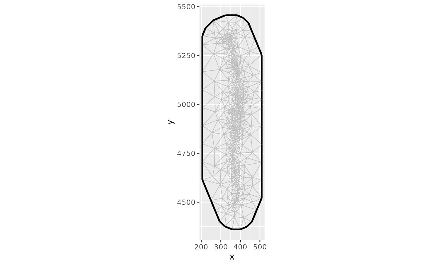
The QQ plot (appearing as a single plot when a non-delta family is used, or 2 plots when a delta family is used) is accessed with
diagnostics$qq_plot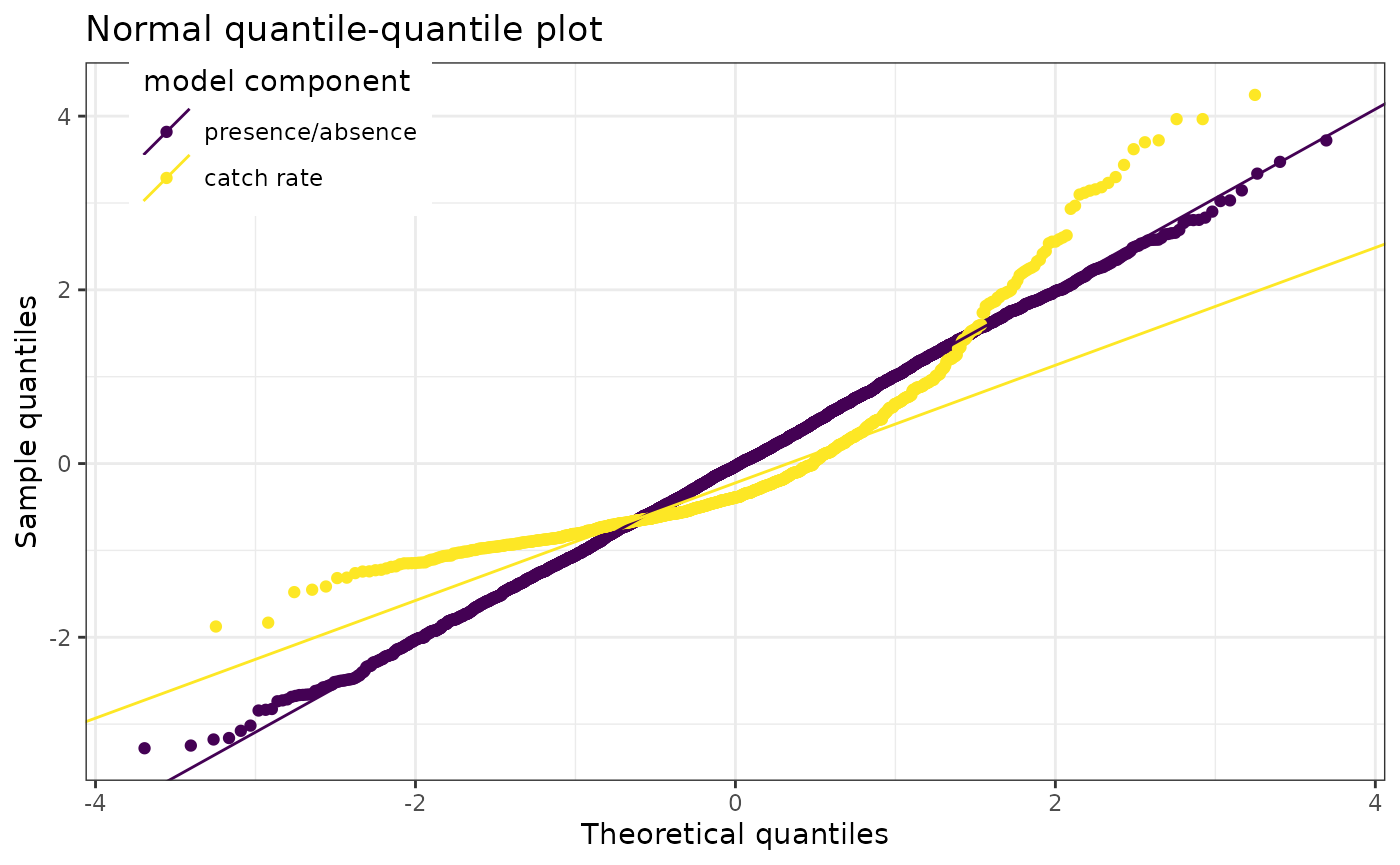
When anisotropy is not included (as in our model) no plot is available, but when included it can be seen by accessing
diagnostics$anisotropy_plot
#> NULL
A plot of the fixed effects parameters can be accessed with
diagnostics$fixed_effects_plot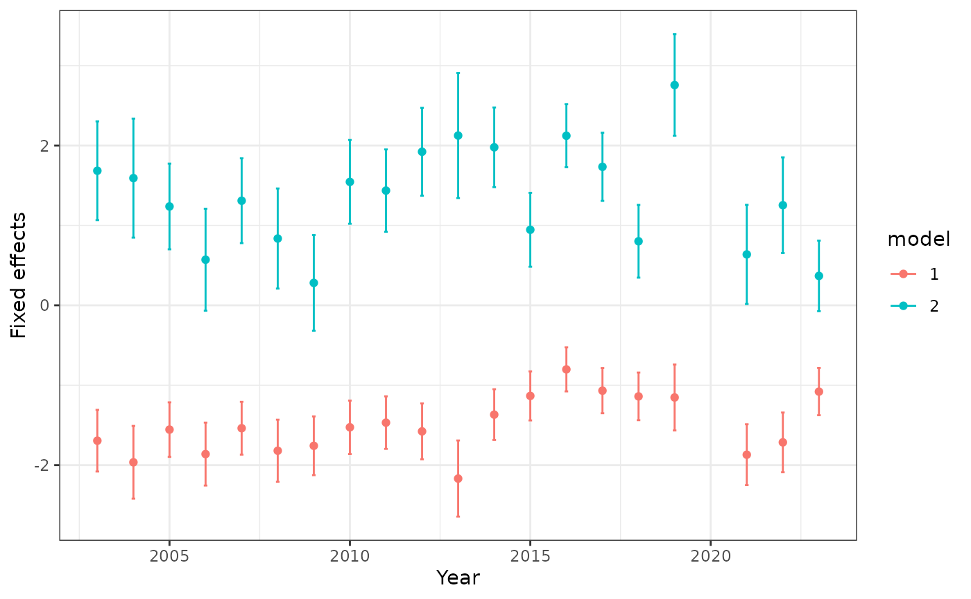
Density plots are made separately for each year, and stored 2 per page in a list of lists. They can be accessed with
diagnostics$density_plots[[10]]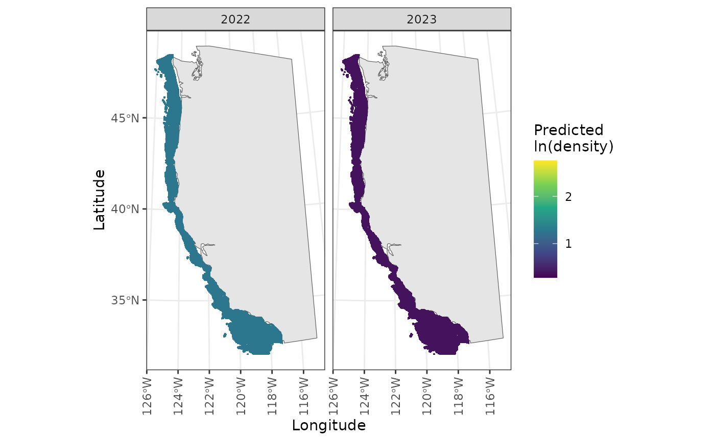
Maps are also made of the residuals. Accessing these can be a little funny, but is done with pagination
plot1 <- diagnostics$residual_maps_by_year[[1]]

ggforce::n_pages(plot1) # check number of pages
#> [1] 10
# View page 2
print(plot1 + ggforce::facet_wrap_paginate("year", nrow = 1, ncol = 2, page = 2))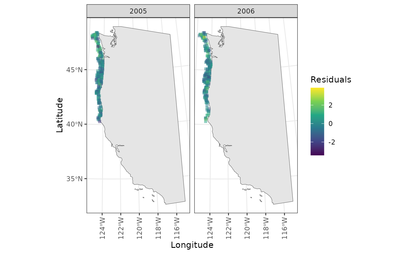
For reproducibility, the diagnostics list also includes a time stamp
diagnostics$date
#> [1] "2026-02-06"
and the session info with
diagnostics$session_info
#> R version 4.5.2 (2025-10-31)
#> Platform: x86_64-pc-linux-gnu
#> Running under: Ubuntu 24.04.3 LTS
#>
#> Matrix products: default
#> BLAS:   /usr/lib/x86_64-linux-gnu/openblas-pthread/libblas.so.3
#> LAPACK: /usr/lib/x86_64-linux-gnu/openblas-pthread/libopenblasp-r0.3.26.so;  LAPACK version 3.12.0
#>
#> locale:
#>  [1] LC_CTYPE=C.UTF-8       LC_NUMERIC=C           LC_TIME=C.UTF-8
#>  [4] LC_COLLATE=C.UTF-8     LC_MONETARY=C.UTF-8    LC_MESSAGES=C.UTF-8
#>  [7] LC_PAPER=C.UTF-8       LC_NAME=C              LC_ADDRESS=C
#> [10] LC_TELEPHONE=C         LC_MEASUREMENT=C.UTF-8 LC_IDENTIFICATION=C
#>
#> time zone: UTC
#> tzcode source: system (glibc)
#>
#> attached base packages:
#> [1] stats     graphics  grDevices utils     datasets  methods   base
#>
#> other attached packages:
#> [1] tibble_3.3.1 sdmTMB_1.0.0 purrr_1.2.1  indexwc_0.8  dplyr_1.2.0
#>
#> loaded via a namespace (and not attached):
#>  [1] gtable_0.3.6       raster_3.6-32      TMB_1.9.19         xfun_0.56
#>  [5] bslib_0.10.0       ggplot2_4.0.2      htmlwidgets_1.6.4  lattice_0.22-7
#>  [9] vctrs_0.7.1        tools_4.5.2        Rdpack_2.6.5       generics_0.1.4
#> [13] proxy_0.4-29       pkgconfig_2.0.3    Matrix_1.7-4       KernSmooth_2.23-26
#> [17] RColorBrewer_1.1-3 S7_0.2.1           desc_1.4.3         assertthat_0.2.1
#> [21] lifecycle_1.0.5    compiler_4.5.2     farver_2.1.2       fmesher_0.6.1
#> [25] textshaping_1.0.4  terra_1.8-93       ggforce_0.5.0      codetools_0.2-20
#> [29] htmltools_0.5.9    class_7.3-23       sass_0.4.10        yaml_2.3.12
#> [33] pillar_1.11.1      pkgdown_2.2.0      jquerylib_0.1.4    tidyr_1.3.2
#> [37] MASS_7.3-65        classInt_0.4-11    cachem_1.1.0       wk_0.9.5
#> [41] viridis_0.6.5      reformulas_0.4.4   nlme_3.1-168       inlabru_2.13.0
#> [45] tidyselect_1.2.1   digest_0.6.39      sf_1.0-24          labeling_0.4.3
#> [49] splines_4.5.2      polyclip_1.10-7    rprojroot_2.1.1    fastmap_1.2.0
#> [53] grid_4.5.2         here_1.0.2         cli_3.6.5          magrittr_2.0.4
#> [57] broom_1.0.12       e1071_1.7-17       withr_3.0.2        scales_1.4.0
#> [61] backports_1.5.0    sp_2.2-0           rmarkdown_2.30     otel_0.2.0
#> [65] gridExtra_2.3      ragg_1.5.0         evaluate_1.0.5     knitr_1.51
#> [69] rbibutils_2.4.1    viridisLite_0.4.3  s2_1.1.9           mgcv_1.9-3
#> [73] rlang_1.1.7        Rcpp_1.1.1         glue_1.8.0         DBI_1.2.3
#> [77] tweenr_2.0.3       jsonlite_2.0.0     R6_2.6.1           systemfonts_1.3.1
#> [81] fs_1.6.6           units_1.0-0
The original data is returned (with residual values added) as
diagnostics$data_with_residuals
#> # A tibble: 4,521 × 21
#>     year fyear survey_name common_name         catch_numbers catch_weight effort
#>    <int> <fct> <chr>       <chr>                       <dbl>        <dbl>  <dbl>
#>  1  2003 2003  WCGBTS      yellowtail rockfish             0        0     0.0177
#>  2  2003 2003  WCGBTS      yellowtail rockfish           703        1.13  0.0196
#>  3  2003 2003  WCGBTS      yellowtail rockfish             0        0     0.0224
#>  4  2003 2003  WCGBTS      yellowtail rockfish             0        0     0.0207
#>  5  2003 2003  WCGBTS      yellowtail rockfish             0        0     0.0187
#>  6  2003 2003  WCGBTS      yellowtail rockfish           186        0.248 0.0209
#>  7  2003 2003  WCGBTS      yellowtail rockfish             0        0     0.0216
#>  8  2003 2003  WCGBTS      yellowtail rockfish             0        0     0.0225
#>  9  2003 2003  WCGBTS      yellowtail rockfish             0        0     0.0175
#> 10  2003 2003  WCGBTS      yellowtail rockfish             0        0     0.0201
#> # ℹ 4,511 more rows
#> # ℹ 14 more variables: pass_scaled <dbl>, vessel_year <fct>, longitude <dbl>,
#> #   latitude <dbl>, depth <dbl>, depth_scaled <dbl[,1]>,
#> #   depth_scaled_squared <dbl[,1]>, x <dbl>, y <dbl>, split_mendocino <chr>,
#> #   residuals <dbl>, residuals2 <dbl>, X <dbl>, Y <dbl>
Finally, predictions on the survey grid (or other data passed in) are stored in a dataframe
diagnostics$predictions
#> # A tibble: 912,560 × 60
#> # Rowwise:
#>    OBJECTID Point_id Northin_m Easting_m latitude longitude Ngdc_m  Hard Mixed
#>       <int>    <int>     <int>     <int>    <dbl>     <dbl>  <int> <dbl> <dbl>
#>  1        1    43127      4000    581500     32.0     -120.  -1414    NA    NA
#>  2        2    43128      4000    583500     32.0     -120.  -1692    NA    NA
#>  3        3    43129      4000    585500     32.0     -120.  -1508    NA    NA
#>  4        4    43130      4000    587500     32.0     -120.  -1324    NA    NA
#>  5        5    43131      4000    589500     32.0     -119.  -1160    NA    NA
#>  6        6    43132      4000    591500     32.0     -119.  -1205    NA    NA
#>  7        7    43133      4000    619500     32.0     -119.  -1600    NA    NA
#>  8        8    43134      4000    621500     32.0     -119.  -1573    NA    NA
#>  9        9    43135      4000    623500     32.0     -119.  -1637    NA    NA
#> 10       10    43136      4000    625500     32.0     -119.  -1568    NA    NA
#> # ℹ 912,550 more rows
#> # ℹ 51 more variables: Soft <dbl>, Slope <fct>, Substrate <int>,
#> #   Confidence <int>, Grain <dbl>, Srtm_m <int>, Rock_dist_ <int>,
#> #   Temp03krig <dbl>, Temp04krig <dbl>, Temp05krig <dbl>, Temp06krig <dbl>,
#> #   Temp07krig <dbl>, Temp08krig <dbl>, Temp09krig <dbl>, Temp10krig <dbl>,
#> #   Temp11krig <dbl>, Tempallyr <dbl>, Cowcod <int>, propInCCA <dbl>,
#> #   propInWCGBTS <dbl>, propInTriennial <dbl>, propInSlope98_00 <dbl>, …
Calculating indices
Last, we can use the calc_index_areas function to
calculate indices, with associated uncertainty. We can calculate areas
for any region in the following list:
available_areas()
#>  [1] "Coastwide"                 "WA"
#>  [3] "OR"                        "CA"
#>  [5] "North of Point Conception" "South of Point Conception"
#>  [7] "North of Cape Mendocino"   "South of Cape Mendocino"
#>  [9] "North of Monterey Bay"     "South of Monterey Bay"
By default, the Coastwide index and 3 state indices are generated, but these indices may be calculated simultaneously (note: there is not really a speed up of doing several at the same time, because they are done sequentially). Again we’ll leave the ‘dir’ argument set to NULL and return everything
index <- calc_index_areas(
  data = fit_simple$data,
  fit = fit_simple,
  prediction_grid = pred_grid,
  boundaries = c("Coastwide"),
  dir = NULL
)
The indices may be visualized by extracting the time series plot
index$plot_indices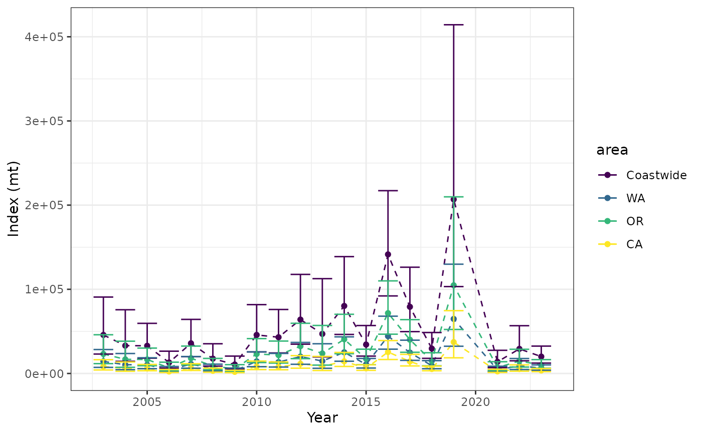
or more custom code could be used to make a plot based off of
index$indices
#>         area year        est         lwr        upr   log_est        se
#> 1  Coastwide 2003  45776.204  23080.8171  90787.983 10.731520 0.3493751
#> 2  Coastwide 2004  33066.659  14444.4891  75696.961 10.406281 0.4225652
#> 3  Coastwide 2005  32881.305  18155.7586  59550.265 10.400660 0.3030242
#> 4  Coastwide 2006  13025.652   6409.1224  26472.832  9.474676 0.3618425
#> 5  Coastwide 2007  35819.918  19968.1294  64255.721 10.486259 0.2981517
#> 6  Coastwide 2008  17604.221   8779.0919  35300.757  9.775894 0.3549890
#> 7  Coastwide 2009  10652.964   5495.7664  20649.649  9.273593 0.3376900
#> 8  Coastwide 2010  45785.712  25636.7911  81770.429 10.731727 0.2958950
#> 9  Coastwide 2011  43052.639  24379.2254  76029.066 10.670179 0.2901544
#> 10 Coastwide 2012  64019.558  34820.4069 117704.077 11.066944 0.3107123
#> 11 Coastwide 2013  47017.098  19626.4773 112633.943 10.758267 0.4457387
#> 12 Coastwide 2014  80231.052  46372.3624 138811.596 11.292666 0.2797026
#> 13 Coastwide 2015  34300.859  20654.4247  56963.529 10.442926 0.2588011
#> 14 Coastwide 2016 141452.302  92131.7924 217175.343 11.859718 0.2187502
#> 15 Coastwide 2017  79215.503  49711.0954 126231.295 11.279927 0.2377308
#> 16 Coastwide 2018  29560.544  17966.3063  48636.919 10.294196 0.2540569
#> 17 Coastwide 2019 206798.126 103227.6334 414283.109 12.239498 0.3544996
#> 18 Coastwide 2021  13823.626   6943.0633  27522.814  9.534134 0.3513514
#> 19 Coastwide 2022  29214.635  15041.7082  56741.886 10.282425 0.3387016
#> 20 Coastwide 2023  20043.525  12352.7782  32522.472  9.905661 0.2469561
#> 21        WA 2003  14344.548   7232.6639  28449.555  9.571125 0.3493751
#> 22        WA 2004  10361.853   4526.3621  23720.594  9.245886 0.4225652
#> 23        WA 2005  10303.770   5689.3350  18660.824  9.240265 0.3030242
#> 24        WA 2006   4081.752   2008.3790   8295.594  8.314282 0.3618425
#> 25        WA 2007  11224.621   6257.2641  20135.337  9.325865 0.2981517
#> 26        WA 2008   5516.504   2751.0387  11061.936  8.615500 0.3549890
#> 27        WA 2009   3338.240   1722.1674   6470.827  8.113199 0.3376900
#> 28        WA 2010  14347.528   8033.6105  25623.791  9.571333 0.2958950
#> 29        WA 2011  13491.085   7639.5365  23824.663  9.509784 0.2901544
#> 30        WA 2012  20061.333  10911.4119  36884.051  9.906549 0.3107123
#> 31        WA 2013  14733.398   6150.2032  35295.261  9.597872 0.4457387
#> 32        WA 2014  25141.408  14531.3622  43498.357 10.132271 0.2797026
#> 33        WA 2015  10748.605   6472.3234  17850.237  9.282531 0.2588011
#> 34        WA 2016  44325.855  28870.6544  68054.622 10.699323 0.2187502
#> 35        WA 2017  24823.173  15577.5961  39556.162 10.119533 0.2377308
#> 36        WA 2018   9263.168   5629.9677  15240.990  9.133801 0.2540569
#> 37        WA 2019  64802.790  32347.6755 129820.816 11.079104 0.3544996
#> 38        WA 2021   4331.807   2175.6961   8624.619  8.373740 0.3513514
#> 39        WA 2022   9154.773   4713.5082  17780.783  9.122031 0.3387016
#> 40        WA 2023   6280.890   3870.8982  10191.325  8.745267 0.2469561
#> 41        OR 2003  23187.711  11691.4744  45988.206 10.051378 0.3493751
#> 42        OR 2004  16749.753   7316.7849  38343.923  9.726139 0.4225652
#> 43        OR 2005  16655.863   9196.7102  30164.894  9.720518 0.3030242
#> 44        OR 2006   6598.080   3246.5094  13409.683  8.794534 0.3618425
#> 45        OR 2007  18144.403  10114.7577  32548.420  9.806117 0.2981517
#> 46        OR 2008   8917.331   4447.0058  17881.425  9.095752 0.3549890
#> 47        OR 2009   5396.207   2783.8534  10459.978  8.593452 0.3376900
#> 48        OR 2010  23192.527  12986.1904  41420.409 10.051585 0.2958950
#> 49        OR 2011  21808.103  12349.1767  38512.149  9.990037 0.2901544
#> 50        OR 2012  32428.792  17638.1058  59622.421 10.386802 0.3107123
#> 51        OR 2013  23816.280   9941.6956  57054.170 10.078125 0.4457387
#> 52        OR 2014  40640.645  23489.6921  70314.331 10.612524 0.2797026
#> 53        OR 2015  17374.931  10462.3972  28854.595  9.762784 0.2588011
#> 54        OR 2016  71651.968  46668.9063 110009.102 11.179576 0.2187502
#> 55        OR 2017  40126.223  25180.9109  63941.841 10.599785 0.2377308
#> 56        OR 2018  14973.748   9100.7441  24636.792  9.614054 0.2540569
#> 57        OR 2019 104752.573  52289.4499 209853.071 11.559356 0.3544996
#> 58        OR 2021   7002.290   3516.9746  13941.546  8.853992 0.3513514
#> 59        OR 2022  14798.530   7619.3033  28742.323  9.602283 0.3387016
#> 60        OR 2023  10152.949   6257.2391  16474.098  9.225519 0.2469561
#> 61        CA 2003   8243.944   4156.6788  16350.222  9.017234 0.3493751
#> 62        CA 2004   5955.053   2601.3421  13632.444  8.691995 0.4225652
#> 63        CA 2005   5921.672   3269.7134  10724.548  8.686374 0.3030242
#> 64        CA 2006   2345.820   1154.2340   4767.555  7.760390 0.3618425
#> 65        CA 2007   6450.894   3596.1075  11571.964  8.771974 0.2981517
#> 66        CA 2008   3170.386   1581.0474   6357.397  8.061609 0.3549890
#> 67        CA 2009   1918.517    989.7455   3718.844  7.559308 0.3376900
#> 68        CA 2010   8245.657   4616.9902  14726.229  9.017442 0.2958950
#> 69        CA 2011   7753.451   4390.5122  13692.254  8.955893 0.2901544
#> 70        CA 2012  11529.433   6270.8892  21197.605  9.352658 0.3107123
#> 71        CA 2013   8467.420   3534.5786  20284.512  9.043981 0.4457387
#> 72        CA 2014  14448.999   8351.3081  24998.908  9.578380 0.2797026
#> 73        CA 2015   6177.323   3719.7041  10258.696  8.728640 0.2588011
#> 74        CA 2016  25474.479  16592.2318  39111.620 10.145432 0.2187502
#> 75        CA 2017  14266.107   8952.5884  22733.292  9.565642 0.2377308
#> 76        CA 2018   5323.628   3235.5945   8759.138  8.579910 0.2540569
#> 77        CA 2019  37242.762  18590.5080  74609.222 10.525213 0.3544996
#> 78        CA 2021   2489.529   1250.3926   4956.648  7.819849 0.3513514
#> 79        CA 2022   5261.333   2708.8967  10218.780  8.568140 0.3387016
#> 80        CA 2023   3609.686   2224.6410   5857.049  8.191376 0.2469561
#>    se_natural  type
#> 1   45776.204 index
#> 2   33066.659 index
#> 3   32881.305 index
#> 4   13025.652 index
#> 5   35819.918 index
#> 6   17604.221 index
#> 7   10652.964 index
#> 8   45785.712 index
#> 9   43052.639 index
#> 10  64019.558 index
#> 11  47017.098 index
#> 12  80231.052 index
#> 13  34300.859 index
#> 14 141452.302 index
#> 15  79215.503 index
#> 16  29560.544 index
#> 17 206798.126 index
#> 18  13823.626 index
#> 19  29214.635 index
#> 20  20043.525 index
#> 21  14344.548 index
#> 22  10361.853 index
#> 23  10303.770 index
#> 24   4081.752 index
#> 25  11224.621 index
#> 26   5516.504 index
#> 27   3338.240 index
#> 28  14347.528 index
#> 29  13491.085 index
#> 30  20061.333 index
#> 31  14733.398 index
#> 32  25141.408 index
#> 33  10748.605 index
#> 34  44325.855 index
#> 35  24823.173 index
#> 36   9263.168 index
#> 37  64802.790 index
#> 38   4331.807 index
#> 39   9154.773 index
#> 40   6280.890 index
#> 41  23187.711 index
#> 42  16749.753 index
#> 43  16655.863 index
#> 44   6598.080 index
#> 45  18144.403 index
#> 46   8917.331 index
#> 47   5396.207 index
#> 48  23192.527 index
#> 49  21808.103 index
#> 50  32428.792 index
#> 51  23816.280 index
#> 52  40640.645 index
#> 53  17374.931 index
#> 54  71651.968 index
#> 55  40126.223 index
#> 56  14973.748 index
#> 57 104752.573 index
#> 58   7002.290 index
#> 59  14798.530 index
#> 60  10152.949 index
#> 61   8243.944 index
#> 62   5955.053 index
#> 63   5921.672 index
#> 64   2345.820 index
#> 65   6450.894 index
#> 66   3170.386 index
#> 67   1918.517 index
#> 68   8245.657 index
#> 69   7753.451 index
#> 70  11529.433 index
#> 71   8467.420 index
#> 72  14448.999 index
#> 73   6177.323 index
#> 74  25474.479 index
#> 75  14266.107 index
#> 76   5323.628 index
#> 77  37242.762 index
#> 78   2489.529 index
#> 79   5261.333 index
#> 80   3609.686 index
Saving output
As demonstrated above, there are a lot of plots and diagnostics that
can be inspected, and in many cases we might want to save everything.
The save_index_outputs function in indexwc
will write everything locally (for the directory structure, see
?save_index_outputs)
save_index_outputs(
  fit = fit_simple,
  diagnostics = diagnostics,
  indices = index,
  dir_main = paste0(getwd(), "/yellowtail_example")
)